Overview

Installation

Prerequisites:

Before you begin, ensure that Conda is installed on your system. You can download and install either Anaconda or the lighter Miniconda distribution.

Step 1: Clone the Repository

Clone the repository to your local machine:

git clone https://github.com/cci-MaLab/Calcium-Transient-Analysis.git
cd Calcium-Transient-Analysis

Step 2: Create the Conda Environment

For full functionality including machine learning support with PyTorch, create the environment using the provided YAML file:

conda env create -f environment_ml.yml

If you do not require the machine learning parts of the GUI (which include PyTorch and have larger install requirements), you can create a lighter environment instead:

conda env create -f environment_basic.yml

Note

The environment name is specified in the YAML file under the name: field. It will be set to cell_exploration_ml or cell_exploration depending on which aformentioned .yml file was picked. We will assume here that environment_ml.yml was used for the rest of the guide.

Step 3: Activate the Environment

After creating the environment, activate it with:

conda activate cell_exploration_ml

Step 4: Run the Application

With the environment activated, run the main application by executing:

python main.py

On subsequent runs, you will only need to activate the environment and run the application, a.k.a. steps 3 and 4.

Alternative: Using pip

If you prefer pip over conda, we provide a requirements file for a basic installation:

pip install -r requirements_basic.txt

Demo Data

You can test the GUI out with demo data provided at this link.

Main Window

Before you use the GUI ensure that your data is set up correctly in their corresponding folders and that the config file points to the correct directories. Please refer to Creating the Config File and Video files for more information.

Once the GUI is loaded you should see the following window:

To load in a specific dataset, click File -> Load Data then proceed to select the config file you have created in Creating the Config File. You can also load in other datasets as well and their corresponding max projection of cell footprints will be visualized. If you wish to save the currently loaded setup of datasets, click File -> Save, this will create a json file that will point to all loaded config.ini files. To load in a saved setup, click File -> Load Saved State. Below is an example of what a generated json file could look like:

{
    "C:/Users/Michal Lange/Documents/Calcium-Transient-Analysis/config_files/configA58S4.ini": null,
    "C:/Users/Michal Lange/Documents/Calcium-Transient-Analysis/config_files/configA34D1S1.ini": null,
    "defaults": {
        "ALP": {
            "window": 20,
            "delay": 0
        },
        "ILP": {
            "window": 20,
            "delay": 0
        },
        "RNF": {
            "window": 20,
            "delay": 0
        },
        "ALP_Timeout": {
            "window": 20,
            "delay": 0
        },
        "distance_metric": "euclidean"
    }
}

The defaults and distance_metric parts can be ignored as they are utilized for the cell clustering part of the GUI and is not part of CalTrig. File paths can be added or removed as needed from the json file, however it is recommended to use the GUI to save and load the state to avoid any issues.

CalTrig

In order to use the CalTrig utility, select a given dataset from the main window view, switch to the CalTrig tab and click Start CalTrig.

This will open a new window for the specified dataset that will look like this:

For the time being let’s focus on the upper half part of the window. The upper section is primarily occupied by the visualization of the video, with tools underneath for playing and scrolling the video. You can move the video view by clicking and dragging your mouse, you can also zoom in on any part of the video with the scroll wheel. You can also switch between different video types by right-clicking on the video and selecting Video Format.

To the right of the video you have a series of tabs with differing functionality:

Approved Cells - Initially all cells are considered approved and it is up to the user to verify or reject them. Select any number of cells from the list (use ctrl to select multiple or ctrl+a to select all) and click on Focus Selection to see the selection visualized on the video, or click Focus and Trace to simultaneously visualize the selection and immediately plot the corresponding traces in the lower half of the window. You can revert back to the original state by pressing Reset Mask. Once cells have been selected you can click on them individually to have their corresponding traces visualized on the lower half of the window.

The Highlight Mode dropdown controls how selected cells are drawn on the video: Outline draws a border around each cell footprint, Color fills the footprint, and Clear removes all highlighting without resetting the selection.

The Verify/Unverify button highlights the cell in green to indicate it has already been checked. If you notice any issue with an observed cell, press Reject Cell(s) to move it to the rejected list.

Cells can also be organised into named groups. Select one or more cells and press Add to Group or Remove from Group to manage group membership. Alternatively, right-click on the video and choose Add Group → Rectangle or Add Group → Ellipse to draw a spatial ROI directly on the video; all cell footprints that fall within the drawn shape will be added to a new group automatically.
Rejected Cells - All cells that have been rejected will appear as a list in this tab. If a rejection was made erroneously you can return it by selecting the cell and pressing the Return Cell button. Selecting a cell and pressing Show/Justify Rejection opens a free-text field where a written justification for the rejection can be entered or reviewed; press Save to store the note or Cancel to dismiss without saving.
Missed Cells - The missed cell section provides the ability to the user to highlight any cell that could have been missed by the preprocessing software. Before selecting Enable Select Cell Mode make sure the field of view in the video section is zoomed in on the section where you have detected a missing cell. In Enable Select Cell Mode the field of view will be frozen, allowing the user to trace out the outlines of a cell by holding down the left-mouse button. If the outline is completed and the drawn trace is closed, the inner part of the trace will be filled as well. A right-mouse click and drag will remove any selected pixels. Once completed press Confirm Selected Pixels to add the selection to the Missed Cells list. The selection of the missed cell will generate a signal based on the sum of the pixel values across time using the raw signal from the processed video array.

Between the lower and upper half of the window there is a divider which can be dragged to adjust the size of the respective halves.

Once a signal is selected its corresponding trace can be seen in the bottom half of the window. This plot is similarly interactable like the video in the upper half (click-and-drag to pan, scroll to zoom); the axes can also be zoomed independently by holding down the right mouse button and dragging. To the right of the trace is a panel with three tabs:

Params

Contains four sub-tabs for adjusting how the signal is displayed and analysed:

SavGol — applies a Savitzky-Golay smoothing filter to the ΔF/F signal. Set Window Length, Polynomial Order, Derivative, and Delta, then press Update SavGol to redraw the trace.
Noise — overlays a rolling noise baseline on the trace. Choose a Window Length, a Type (None / Mean / Median / Max), and a Cap value, then press Update Noise.
View — controls the visible range of the trace plot. Set Y Axis Start and Y Axis End to fix the vertical range, and Window Size to limit how many frames are shown at once. Enable Single Plot View to stack all selected cells’ traces with configurable Inter Cell Distance and Intra Cell Distance spacing. Press Update View to apply.
Window Size Preview — draws a preview window on the trace before committing to a window size for analysis. Set a Window Size, divide it into subwindows using the No. of Subwindows slider, and adjust a Lag offset. Tick Preview to overlay it live on the trace, or tick Event Window and select an event type (RNF / ALP / ILP / ALP_Timeout) from the dropdown to align the preview to that event. Press Update Size to set the window.

Above the sub-tabs is a set of signal checkboxes that toggle which trace types are overlaid on the plot: C Signal (white), S Signal (magenta), Raw Signal (cyan), ΔF/F (yellow), SavGol Filter (ΔF/F) (yellow-green), Noise (light blue), and SNR (pink). Behavioural event markers (RNF, ALP, ILP, ALP_Timeout) are also available as overlays when present in the loaded dataset.

Event Detection

Contains up to three sub-tabs for creating and reviewing transient events:

Automatic — set a Peak Threshold (ΔF/F), an Interval Threshold (frames), and an SNR Threshold, then press Calculate Events to run peak detection on the selected cell. If a trained model file is available, a model selector dropdown and Run Model button also appear here. Select the desired model, set the Model Confidence Threshold (default 0.5), and press Run Model. The model’s predicted events appear as temporary picks highlighted on the trace. Use Toggle Temp Picks to show or hide them and Show Evaluation Metrics to inspect performance statistics. Choose a confirmation mode — Accept Incoming Only (only picks that do not overlap with existing events), Accept Overlapping Only (only picks that coincide with existing ones), or Accept All — then press Confirm Temp Picks (green) to finalise or Clear Temp Picks (red) to discard.
Manual — provides tools for hand-crafting events. Double-click two points on the trace to mark the start and end of a candidate transient, then press Create Event to confirm it as a red segment. To remove an event, click the red segment to turn it blue, then press Clear Selected Events. The Force/Readjust Transient Event tool lets you type an exact Start and End frame and press the active button to snap an existing event to those bounds.
ML Results (only visible when pre-loaded test result files are present) — displays evaluation comparisons between pre-computed ML run results and manual annotations. Use the dropdowns to select the experiment, testing set, and number of cells, then press Generate ML Results to produce the comparison.

Local Stats

Press Generate Local Statistics to produce amplitude and inter-event interval (IEI) distributions for the currently selected cell.

Session Settings

Visualization and analysis parameters can be persisted across sessions without re-entering them each time. From the CalTrig menu bar go to Utilities → Save Current Session Settings to export all current parameters (signal types, window sizes, shuffling settings, and more) to a JSON file. To restore a previously saved state, go to Utilities → Load Session Settings and select the corresponding file.

3D & Advanced Visualization

Both 3D views are disabled by default. Enable them from the menu bar via Select Videos/Visualizations → tick 3D Visualization or Advanced 3D Visualization. Each enabled view appears alongside the cell video in the upper panel and can be resized using the horizontal splitter handles between views.

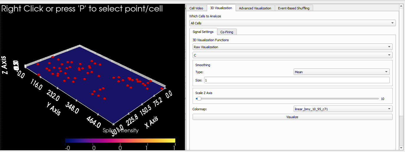
3D Visualization

Reached via the 3D Visualization tab on the right-hand panel, which contains two sub-tabs:

Signal Settings — renders all selected cells as a 3D surface or spike landscape over time. Use the Which Cells to Analyze dropdown (All Cells / Verified Cells / any named Group) to scope the population. Choose a 3D Visualization Function:
- Raw Visualization — plots the raw signal value (C, DFF, or Binary Transient, selected from the data-type dropdown) for each cell continuously over time. When Transient Visualization is chosen additional modifiers appear: Cumulative, Normalize, and Average checkboxes change how the transient signal is accumulated and scaled.
A Smoothing frame controls a rolling mean that is applied before rendering (set Type and Size). The Scale Z Axis slider exaggerates the vertical dimension for easier visual inspection. A Colormap dropdown lets you cycle through all available colormaps. Press Visualize to render the scene.
Co-Firing — described in the Co-Firing & Shuffling section below.

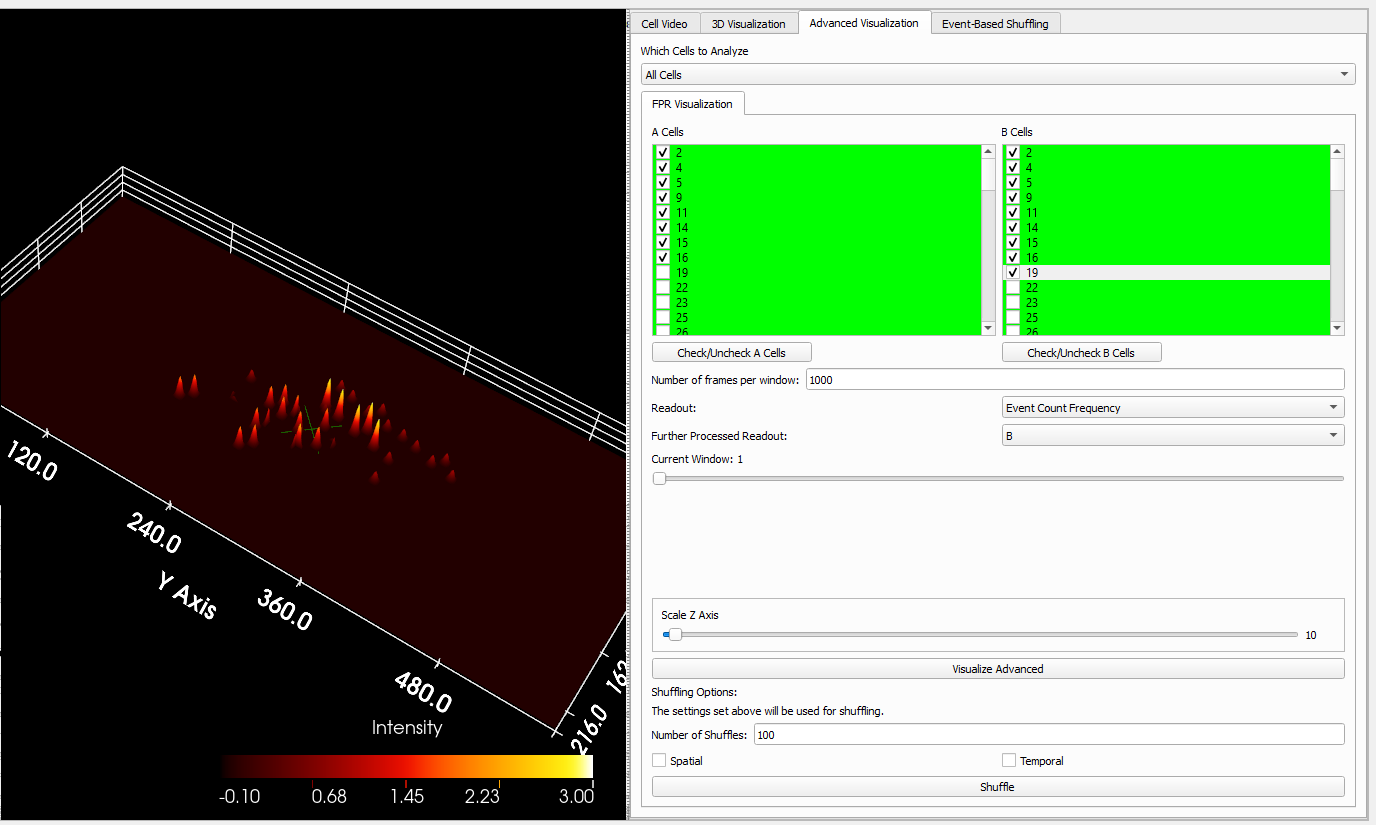
Advanced Visualization

Reached via the Advanced Visualization tab. It compares two populations of cells (A and B) across sliding time windows using a Further Processed Readout (FPR). Select a cell population from the Which Cells to Analyze dropdown, then assign cells to the A Cells and B Cells lists using the checkboxes (or the Check/Uncheck buttons for bulk selection). Configure:

Number of frames per window — the temporal resolution of each window evaluated on the 3D surface.
Readout — the per-window metric computed for each cell: Event Count Frequency, Average DFF Peak, or Total DFF Peak.
Further Processed Readout (FPR) — a formula combining the A and B readouts into a single value displayed on the surface. Options are B, B-A, (B-A)², (B-A)/A, |(B-A)/A|, and B/A.
Scale Z Axis — vertical exaggeration slider.

Press Visualize Advanced to render. A window slider appears below letting you step through each time window.

The Shuffling Options section below the visualize button lets you validate results against chance: tick Spatial, Temporal, or both, set a Number of Shuffles, and press Shuffle. A separate slider appears to step through the shuffled windows for comparison.

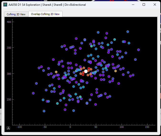
Co-Firing & Shuffling

The Co-Firing sub-tab lives inside the 3D Visualization tab alongside Signal Settings. It overlays co-firing relationships directly on the 3D surface and provides a 2D summary matrix.

Set the Co-Firing Window Size (frames) and press Update Cofiring Window to recalculate which cell pairs fire within that window of each other. The Show Cofiring checkbox toggles the co-firing overlay on the 3D surface.

The Direction dropdown controls which cell must fire first: Bidirectional counts co-firing regardless of order, Forward requires A to fire before B, and Backward requires B before A. Share A and Share B checkboxes control whether the A or B cell in a pair is allowed to appear in multiple co-firing pairs.

Two sub-tabs list participating cells:

Group Co-Firing — shows named cell groups; tick a group to include all its members.
Individual Cells — shows every cell individually; tick any combination for fine-grained control.

Press Show 2D Representation to open a separate matrix window where rows and columns are cells and each entry shows the co-firing count between that pair.

Shuffling

Below the co-firing list is a Shuffling Options section. Select which cells to include via the Select Cells to Shuffle dropdown and the A Cells / B Cells checklists (toggle all with Check/Uncheck buttons). Options:

Verified Cells Only — restricts the shuffled population to verified cells.
Spatial — permutes the spatial positions of cells while keeping timing intact.
Temporal — permutes the inter-event intervals (IEIs) of each cell while keeping spatial positions intact.
No. of Shuffles — number of permutation iterations (default 100).

Press Shuffle to run. A results window opens showing the observed co-firing values against the shuffled null distribution with z-scores for each cell pair.

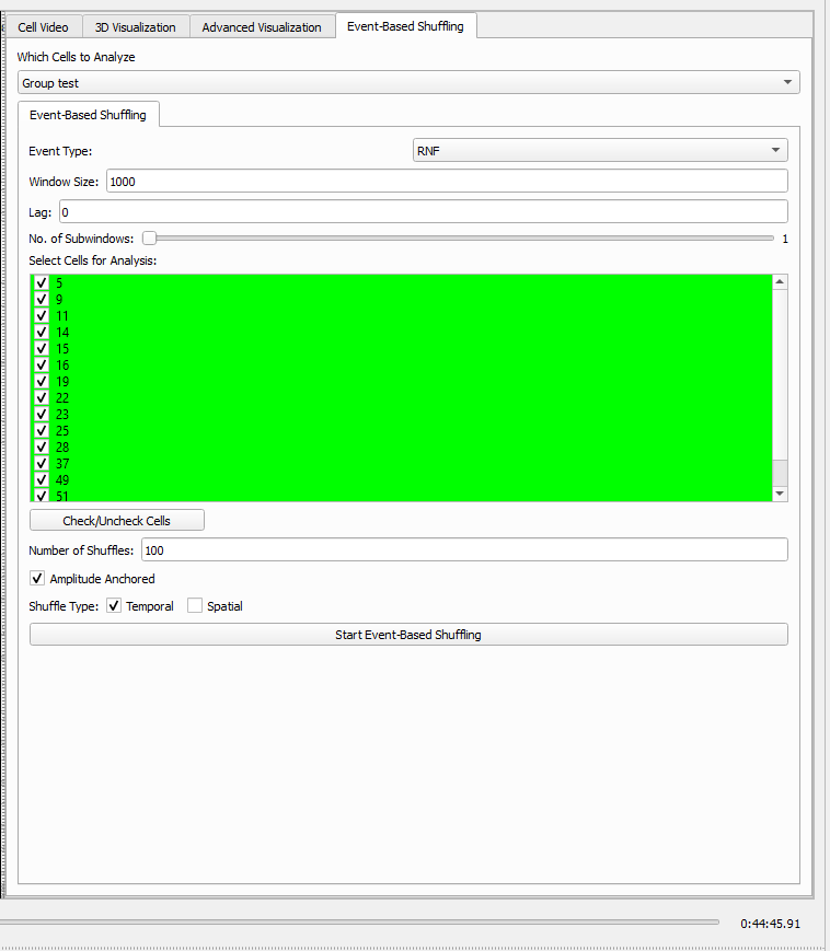
Event-Based Shuffling

The Event-Based Shuffling tab is accessed from the top-level tab strip on the right-hand panel (alongside Cell Video, 3D Visualization, and Advanced Visualization).

This analysis centres each shuffle window around a specific behavioural event type rather than across the full recording. Configure the following parameters before running:

Which Cells to Analyze — All Cells, Verified Cells, or a named Group.
Event Type — the behavioural event to anchor the window: RNF, ALP, ILP, or ALP_Timeout.
Window Size — number of frames on either side of each event occurrence to include.
Lag — frame offset applied to the window start relative to the event timestamp (negative values shift the window earlier).
No. of Subwindows — slider (1–100) that divides the window into equal sub-segments for finer temporal resolution.
Select Cells for Analysis — checklist of individual cells to include; use Check/Uncheck Cells to toggle all at once.
Number of Shuffles — permutation iterations (default 100).
Amplitude Anchored — when ticked, each shuffled event keeps the original ΔF/F amplitude paired with its new timing. When unticked, amplitudes are shuffled independently of timing.
Shuffle Type — tick Temporal to permute IEIs, Spatial to permute cell positions, or both.

Press Start Event-Based Shuffling to run the analysis. A results window opens showing the observed metric against the shuffled null distribution and spatial maps when spatial shuffling is enabled.

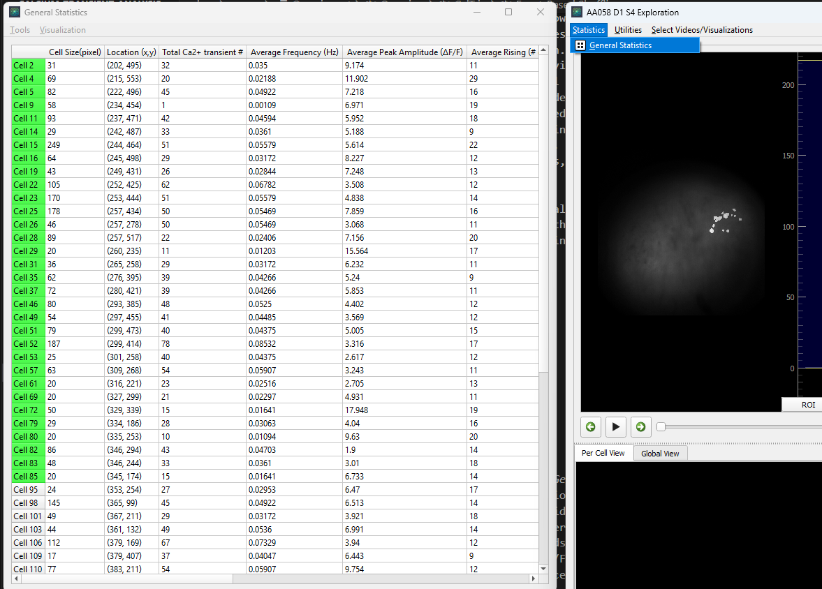
Statistics

General Statistics

From the CalTrig menu bar choose Statistics → General Statistics. This opens a table listing every cell in the session as a row, with the following columns: cell size (pixels), centroid location (x, y), total transient count, average frequency (Hz), average peak amplitude (ΔF/F), average rising duration (frames and seconds), average inter-event interval (frames and seconds), Std(ΔF/F), and MAD(ΔF/F). Row headers are colour-coded: green for verified cells, red for rejected cells.

From the table’s Visualization menu you can generate:

Amplitude Frequency Boxplot — a box plot of average peak amplitudes across all cells.
IEI Frequency Boxplot — a box plot of average inter-event intervals across all cells.

The table can be exported to Excel directly from the window.

Local Statistics

Select a cell and press Generate Local Statistics in the Local Stats tab of the signal panel (see CalTrig). This opens a per-transient table with one row per detected event, listing start and stop frame, duration, interval from the previous transient, peak amplitude, and total amplitude, all in both frames and seconds.

From the table’s Visualization menu:

Amplitude Frequency Histogram — histogram or CDF of total amplitudes for this cell. Set a bin size (ΔF/F) and press Visualize.
ITI Frequency Histogram — histogram or CDF of inter-event intervals (ms). Set a bin size (ms) and press Visualize.
FFT Frequency — FFT of the cell’s ΔF/F trace, showing the dominant oscillation frequencies.

All figures can be saved to SVG, PNG, JPEG, or PDF via the Save Figure button.

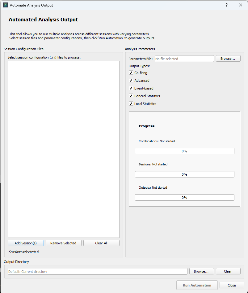
Automation

The automation tool runs the full analysis pipeline across any number of sessions in one go, optionally sweeping over a grid of parameter values. Access it from the CalTrig menu bar via Utilities → Automate Output.

Setting up a run

The dialog has three areas:

Session Configuration Files — add one or more .ini config files (the same type used to load data into the main window) using Add Session(s). Sessions can be removed individually with Remove Selected or cleared all at once with Clear All.
Analysis Parameters — browse to a single JSON file that contains all analysis parameters. This is the same file saved by Save Current Session Settings (see Session Settings). Five Output Types checkboxes control which analyses are written to disk: Co-firing, Advanced, Event-based, General Statistics, and Local Statistics. Untick any output type to skip it.
Output Directory — choose where results are written. If left blank the current working directory is used. Each session produces a sub-folder named <mouseID>_<day>_<session>.

Press Run Automation (enabled only once both sessions and a parameter file have been selected) to start. Three progress bars track combinations, sessions, and individual output types in real time.

Grid search

If any parameter value in the JSON file is supplied as a list with multiple entries (for example "window_size": [500, 1000, 2000]), the automation engine expands all combinations automatically. Each combination gets its own sub-folder inside the session folder, named after the varying parameters and their values. A manifest JSON file is written into each combination folder recording the exact parameters used, making results fully reproducible.